Computing the El Niño index from ERA5 with SQL

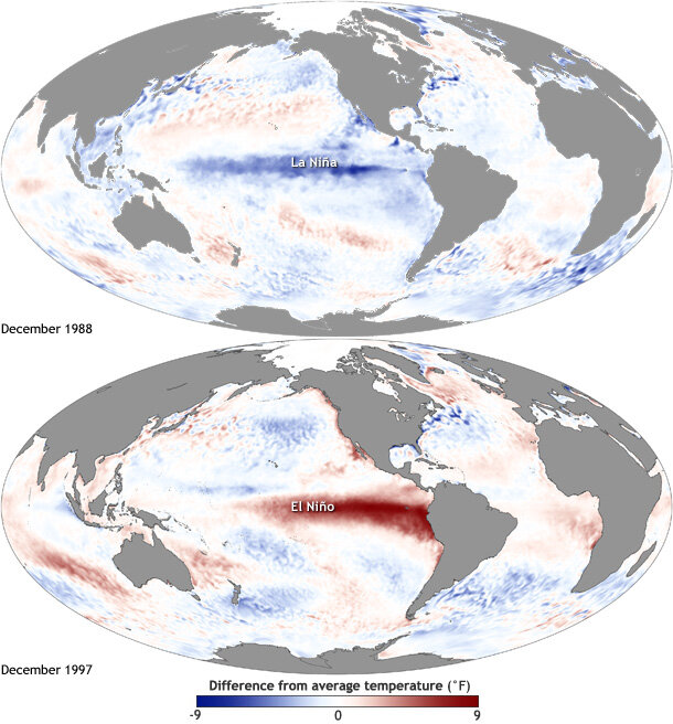
Satellite view of equatorial Pacific sea-surface temperatures during an El Niño event.

Image credit: NOAA Climate.gov

The Oceanic Niño Index (ONI) is the headline number for tracking El Niño and La Niña. When it climbs above +0.5 °C, insurers reprice catastrophe risk, grain traders revise yield forecasts, and energy planners brace for shifted demand. It is one of the most consequential single numbers in climate.

The usual way to compute it: pick a reanalysis dataset, download a multi-decade subset, build an ETL pipeline to reshape it, load it into a warehouse, and finally run the analysis. In this post we skip all of that. We compute the full ONI time series — every 3-month season from 1950 to today — with one SQL query that runs in place against cloud-hosted Zarr, using zarr-datafusion. Nothing gets copied. The compute goes to the data.

By the end, we’ll have validated the result against NOAA’s official table: a mean absolute error of 0.17 °C and a Pearson correlation of 0.966 against a completely independent dataset.

The full, runnable version of everything below — SQL, validation script, and plots — lives in the el-nino-oni cookbook. This post is the narrated tour; the README is the recipe.

What we’re actually computing

The ONI is a 3-month running mean of sea-surface-temperature (SST) anomalies in the Niño-3.4 region of the equatorial Pacific — the box bounded by 5°S–5°N and 170°W–120°W. An “anomaly” means: how much warmer or cooler the ocean is than its normal baseline for that month. Average the anomaly over three consecutive months, and you get one ONI value, classified as:

El Niño when ONI ≥ +0.5 °C
La Niña when ONI ≤ −0.5 °C
Neutral in between

The subtle part is “normal.” NOAA doesn’t use one fixed baseline. It uses a centred, rolling 30-year climatology that shifts forward every five years, so each season is judged against a baseline contemporary to its own decade. A 1960s season is measured against a 1950s–1970s normal; a 2020s season against the 1991–2020 normal. In a warming climate, that’s the difference between measuring ENSO and accidentally measuring the warming trend. Reproducing that schedule faithfully is what keeps our answer honest.

The data: ERA5, queried where it lives

We query ARCO-ERA5, the cloud-optimized, Zarr-formatted copy of ECMWF’s ERA5 reanalysis hosted on Google Cloud. It spans 1940 to the present at 0.25° resolution. We never download it — zarr-datafusion registers it as an external table and reads only the chunks the query touches:

CREATE EXTERNAL TABLE IF NOT EXISTS era5
  STORED AS ZARR
  LOCATION 'gs://gcp-public-data-arco-era5/ar/full_37-1h-0p25deg-chunk-1.zarr-v3';

That single statement turns an 80-year, multi-terabyte climate archive into something you can write SQL against.

Building the query, one step at a time

The whole computation is a chain of CTEs. Let’s assemble it the way you’d actually reason through it.

Step 1 — Sample the Niño-3.4 box. Pull SST from inside the box and convert Kelvin to Celsius. We take a single noon-of-the-15th reading per month: not a true monthly mean, but a cheap, representative sample that keeps the remote read small. Note the discipline in the WHERE clause — we filter only on coordinates (latitude, longitude, time), which is what lets the engine push the filter down to the chunks and avoid scanning the rest of the planet.

WITH samples AS (
  SELECT
    CAST(extract(year  FROM ts) AS INT) AS yr,
    CAST(extract(month FROM ts) AS INT) AS mo,
    sst_c
  FROM (
    SELECT
      arrow_cast(time, 'Timestamp(Microsecond, Some("UTC"))') AS ts,
      sea_surface_temperature - 273.15 AS sst_c
    FROM era5
    WHERE latitude  BETWEEN  -5.0 AND   5.0
      AND longitude BETWEEN 190.0 AND 240.0   -- 170°W–120°W in 0–360° form
  ) AS box
  WHERE extract(day  FROM ts) = 15
    AND extract(hour FROM ts) = 12
    AND extract(year FROM ts) BETWEEN 1940 AND 2026
)

A caveat to be upfront about: this is the biggest approximation in the whole pipeline. A “monthly” value here is built from a single hourly field — 12:00 UTC on the 15th — treated as representative of the entire month. ERA5 actually has hourly data; a faithful monthly mean would average all ~720 hourly steps. We don’t, deliberately: sampling one timestep per month keeps the remote reads small enough to run cheaply. The trade-off is real scatter in the result (you’ll see it in the residuals later), and replacing this with a true monthly average is the single most worthwhile improvement to the query.

Step 2 — Collapse the box to a monthly number. Average all the grid cells in the box per (year, month). The HAVING clause quietly drops months where absent chunks read back as NaN.

monthly AS (
  SELECT yr, mo, AVG(sst_c) AS sst_c
  FROM samples
  GROUP BY yr, mo
  HAVING AVG(sst_c) BETWEEN 0 AND 50
)

Step 3 — Encode NOAA’s rolling baseline schedule. This is the methodological heart. A small lookup table maps each block of season-years to the 30-year base period NOAA uses for it.

base_periods(yr_lo, yr_hi, base_lo, base_hi) AS (
  VALUES
    (1940, 1955, 1936, 1965),
    (1956, 1960, 1941, 1970),
    -- … +5 years each step …
    (2001, 2005, 1986, 2015),
    (2006, 2026, 1991, 2020)   -- held at the latest complete 30-yr period
)

Step 4 — Compute the climatology, then the anomaly. For each base period, find the per-month average SST (the “normal”); then subtract each month’s normal from its observed value. A contiguous month counter t sets up the moving average to come.

clim AS (
  SELECT p.yr_lo, m.mo, AVG(m.sst_c) AS clim_sst
  FROM base_periods p
  JOIN monthly m ON m.yr BETWEEN p.base_lo AND p.base_hi
  GROUP BY p.yr_lo, m.mo
),
anom AS (
  SELECT m.yr, m.mo,
         m.yr * 12 + (m.mo - 1) AS t,
         m.sst_c - c.clim_sst   AS anom
  FROM monthly m
  JOIN base_periods p ON m.yr BETWEEN p.yr_lo AND p.yr_hi
  JOIN clim        c ON c.yr_lo = p.yr_lo AND c.mo = m.mo
)

Step 5 — The 3-month centred average. A self-join stitches each month to its neighbours, averaging the three anomalies into one ONI value. Both neighbours must exist, so the series starts cleanly.

oni AS (
  SELECT c.yr, c.mo,
         (p.anom + c.anom + n.anom) / 3.0 AS oni_raw
  FROM anom c
  JOIN anom p ON p.t = c.t - 1
  JOIN anom n ON n.t = c.t + 1
  WHERE c.yr >= 1950
)

Step 6 — Label and classify. Map each centre month to its season code (DJF, JFM, …) and apply the ±0.5 °C thresholds. That final SELECT is the ONI table — 917 seasons of it.

SELECT o.yr AS year, sl.season,
       ROUND(o.oni_raw, 2) AS oni_c,
       CASE WHEN o.oni_raw >=  0.5 THEN 'El Niño'
            WHEN o.oni_raw <= -0.5 THEN 'La Niña'
            ELSE 'Neutral' END AS enso_phase
FROM oni o
JOIN season_label sl USING (mo)
ORDER BY o.yr, o.mo;

Running it

On cloud infrastructure in the same region as the data, this returns in about 60 seconds. Over a home internet connection it’s a 25–35 minute run pulling several GB of remote reads — the query has to reach back to 1940 so the deep-past climatology has data. Either way, the point stands: there was no download, no warehouse, no pipeline. One SQL file produced a complete, decades-long climate index.

Does it actually hold up?

A fast query is worthless if it’s wrong. So we compare all 916 overlapping seasons against NOAA CPC’s official ONI table — which is built from ERSSTv5, an entirely different dataset from ERA5. Agreement here means the signal is real, not an artifact of one data source.

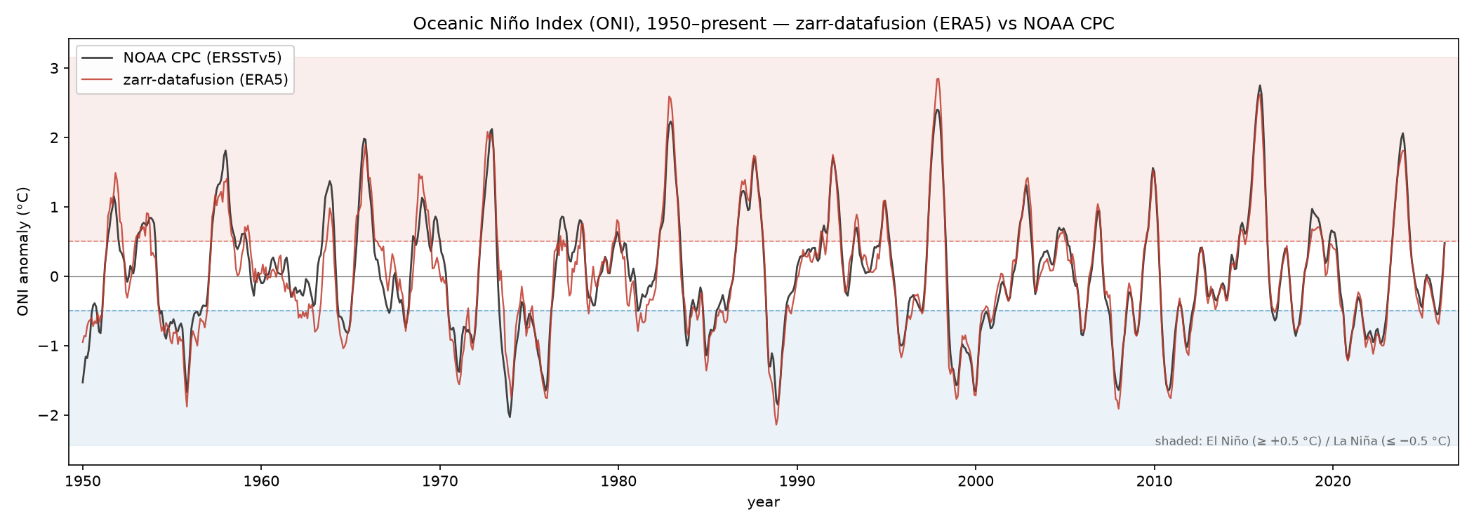
ONI computed from ERA5 (zarr-datafusion) overlaid on NOAA's official ONI, 1950–present — the two lines track tightly across every major El Niño and La Niña event.

The two series track tightly across every major event of the last 75 years. The numbers back up the eye:

Metric	Result
Mean absolute error	0.17 °C overall; 0.12 °C from 1979 on
Pearson correlation	0.966
Systematic bias	−0.04 °C (negligible)
ENSO phase agreement	weighted κ = 0.88, zero sign reversals

Zero sign reversals is the one to sit with: across 916 seasons, the query never once called a warm event cold or a cold event warm. Every disagreement is a single-threshold boundary slip near ±0.5 °C.

Being honest about the error

The residuals aren’t uniform, and that’s the interesting part:

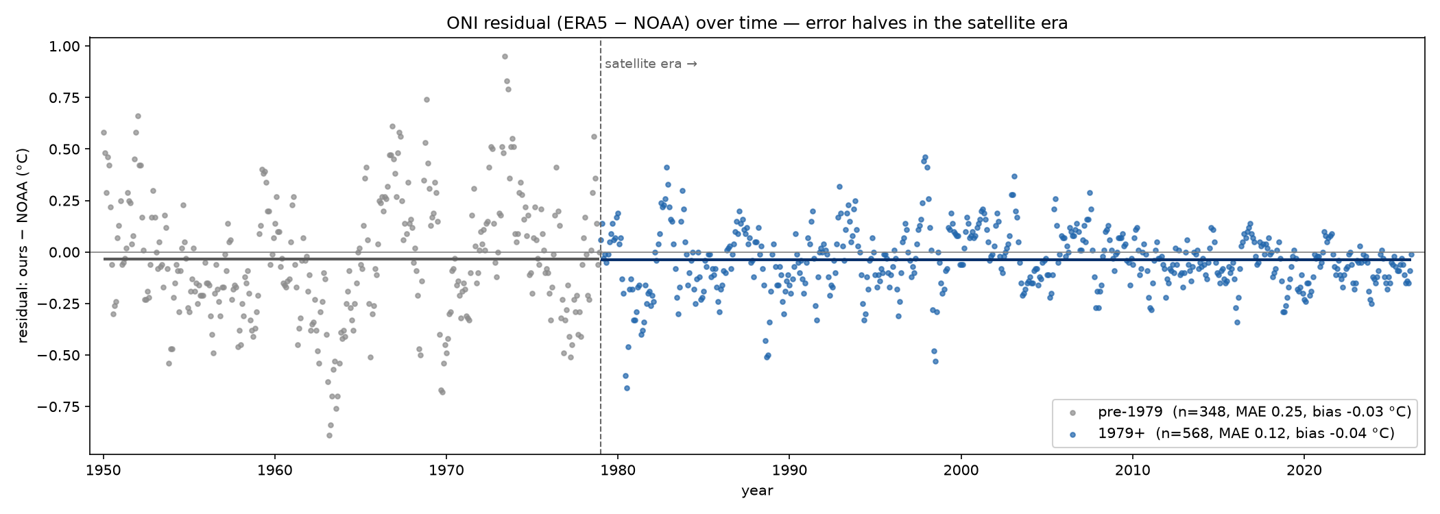
ONI residuals (ERA5 minus NOAA) split by era — error is largest in the 1950s–60s and shrinks steadily toward the present.

Error peaks in the 1960s (0.29 °C) and falls steadily to 0.09 °C by the 2020s. That’s exactly the shape you’d predict: ERA5’s pre-satellite era (before ~1979) is more weakly constrained by observations, so its tropical Pacific SSTs wander further from ERSSTv5. A few other knowingly-accepted sources of scatter:

Dataset mismatch — ERA5 vs. ERSSTv5 carries an inherent ~0.1–0.2 °C difference, which explains most of the residual post-1979.
Sampling shortcut — as flagged above, a single 12:00 UTC reading on the 15th stands in for the whole month instead of a true monthly mean over all hourly steps. This is the largest knob we chose to leave un-tuned, and a meaningful share of the month-to-month scatter comes from it.
Truncated baseline — ARCO-ERA5 starts in 1940, so the earliest 30-year base period (nominally 1936–1965) is really 1940–1965. Unavoidable, and the one place we can’t exactly match NOAA.

None of these are bugs to hide — they’re the honest seams of computing a 75-year index from a single, fast, in-place query.

The takeaway

We reproduced one of climate science’s most-watched indices, validated it against the authoritative independent source, and never moved the data. No ETL job, no warehouse bill, no stale copy to keep in sync — just SQL pointed at a Zarr store in the cloud.

If you want to run it yourself, the cookbook README has every step. And if the question on your mind is less “how” and more “what does this cost to operationalize for climate-risk analytics” — that’s the subject of the companion piece.

If your workflow looks like one of these copy-and-load ETL pipelines, we can help you cut the cost — reach us at [email protected].

References

zarr-datafusion — the SQL engine for Zarr-native array data used throughout this post
el-nino-oni cookbook — full runnable SQL, validation script, and plots
ARCO-ERA5 — the cloud-optimized, Zarr-formatted ERA5 reanalysis queried in place
NOAA CPC — change to ONI base periods — the centred, rolling 30-year climatology schedule
NOAA CPC — official ONI table — the ERSSTv5-based reference we validate against